– Written by Dimple Patel, Clinical Programmer

Growing up in Florida in the 1990s, I hit the jackpot. My sweet primary school teachers were like my adoptive mothers. I’d always hoped those gems would live a hundred years with optimal health, but this past year has been a tough check against my wishful thinking. I lost two teachers: one to a post-surgical cerebrovascular event; the second, to a gastrointestinal adverse event from ibuprofen. As their former student and as a pharmaceutical data scientist, I strive to understand better available CRAN resources – such as the noncompartmental analysis (NCA) R packages – which would streamline pharmacokinetic (PK) analysis to better shape patient outcomes like those of my teachers.

Some of the available NCA R packages include perform pharmacokinetic noncompartmental analysis, PKNCA; noncompartmental analysis for pharmacokinetic data, NonCompart; and noncompartmental pharmacokinetic analysis by qPharmetra, qpNCA. Let’s look at all three noncompartmental analysis packages using sample pharmacokinetic data collected on 12 patients dosed with theophylline, a substance similar to the caffeine I’m sure my teachers imbibed when roughing it in 30-student classrooms!

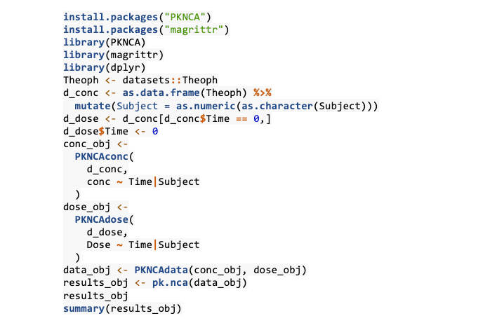
First, I tried out the PKNCA package using the Theoph dataset. Here, the Theoph dataset is fed into as.data.frame function to create an R programming structure that is easier to manipulate – a data frame which is an organised set of vectors. Then the variable ‘Subject’, which is stored in the Theoph dataset as the data type “factor” with 12 levels (denoting 12 patients), is fed into the mutate() function to change its type to numeric.

Then to create the theophylline dosing data, the previous data frame is subsetted using the condition of the concentration of the analyte at time=0 hours, which would act as the initial drug dose. Then three distinct functions come into play: PKNCAconc(), PKNCAdose() and PKNCAdata().

• PKNCAconc() needs two arguments: 1) a time-concentration data frame, d_conc, or another parameter and 2) a formula denoting the relationship where Time (grouped by ‘Subject’) is the independent variable to the dependent variable of conc. PKNCAconc(), which then creates a PKNCAconc object, which will be retrieved later.

• PKNCAdose() requires the same arguments as PKNCAconc(), except the dosing data frame is needed and the formula is specifically written so that ‘conc’ is replaced by ‘Dose’: Dose ~ Time|Subject.

• Both the PKNCAdose object and the PKNCAconc object are merged via the PKNCAdata() method to create a PKNCAdata object, which is then inputted into the function pk.nca(), which calculates the noncompartmental parameters according to user-specified grouping factors (e.g. dose, time).

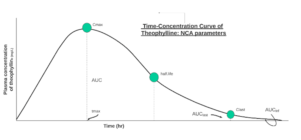
The summary() condenses the data into averages across the patients’ NCA parameters: auclast and aucinf (areas+ under the curve), cmax (maximum concentration), tmax (time at maximum concentration), half.life (time needed for concentration to decrease by half).

The second package, NonCompart, is economic with keystrokes when working with datasets such as the theophylline analyte concentration data. NonCompart’s two main functions are sNCA and tblNCA, which are executed for single patient data and multiple patient data, respectively. In the code below, a straightforward line of code invoked the tblNCA() function with four arguments: concData (concentration data table), key (column names of the concData table shown in the output), dose and concUnit (unit of concentration).

After storing the calculated noncompartmental analysis functions, I invoked the summary() function to distil the otherwise dense results. NonCompart’s tblNCA() function piled up on top of PKNCA’s pk.NCA() function’s outputs of tmax, cmax, auf, etc. with values such as half-life by lambda z (LAMZHL); last positive concentration observed (CLST); area under the moment curve % extrapolated predicted (AUMCPEP); and mean residence time (MRT) using infinity using last concentration predicted (CLSTP) for extravascular administration (MRTEVIFP). Lambda z is the rate at which the drug is removed from the body and is denoted graphically by the slope of the terminal elimination phase.

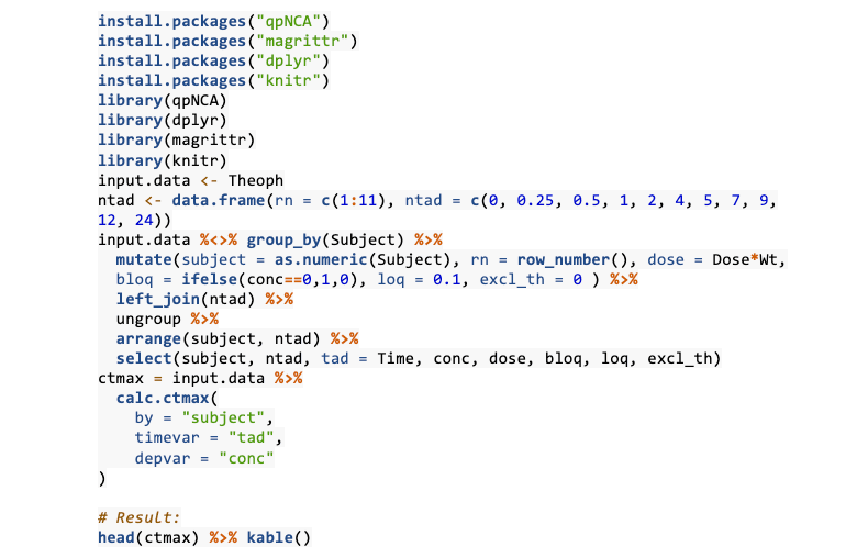
A team of pharmacometric enthusiasts weaved together the third package, qpNCA, which required basic data cleaning and manipulation before step-wise NCA computation. The theophylline dataset is used again with the qpNCA library, which imports the magrittr and the dplyr libraries. The theophylline data is stored in a table input.data. Then, 11 nominal time values are stored in a data frame called ntad. Using the pipe operators via magrittr and basic functions from dplyr, the input.data table is grouped by the variable, Subject.

Then the mutate() function adds new variables such as subject (the numeric form of the group by variable); rn (row_number); dose (the product of dose and weight); bloq (below the limit of quantification variable dependent on dose concentration set to zero); loq (limit of quantification); and excl_th (variable names to be excluded in the half-life calculation) from the input.data table. Then the arrange() function reorders the table’s rows by first subject and then ntad values, and, finally, the select() function culls the variables needed for downstream NCA analysis.

The calc.ctmax() function then works on the cleaned-up input.data table from which it requires three arguments specified: by (grouping variable), timevar (actual post-dose sampling time) and depvar (dependent variable). Knitr’s kable() function then helps output a rectangular table with cmax and tmax values for all 12 subjects. For the terminal half-life of theophylline, several LOQ variables need to be imputed before the qpNCA package’s est.thalf() function can be invoked; this function piles on the base arguments in the calc.ctmax() function with extra variables including exclvar and includeCmax, which controls whether Cmax is included in the half-life estimation.

PKNCA, NonCompart and qpNCA are all powerful R programming packages that can calculate nonparametric analysis parameters with the industrial strength of costly software. PKNCA’s main strengths shine in its thorough vignettes, teaching novice programmers the functionality and PK calculations that the package can handle. Moreover, PKNCA offers clean options through the PKNCA.options commands to users of organisations who may need to adjust the default values for standard parameters and override summarisation methods, which can be modulated by the PKNCA package’s PKNCA.set.summary. Moreover, users can invoke manual interval specification (vs automatic interval control) in the PKNCAdata() function. NonCompart has a similar manual override option in its manual slope selection feature. Moreover, NonCompart supports CDISC SDTM terminology by invoking CDISC-compliant pharmacokinetic parameter (PP) terms in one of its stalwart features, the Unit() function. Although the qpNCA package does not feature any CDISC-mindful functions, the package includes both complete and step-wise instructions for NCA analysis. More impressively, the qpNCA features a whole dossier of background information that explains which PK parameters do not need lambda z; the goings-on in back-extrapolation/interpolation methods; limit of quantification handling; and handling data that may be missing or anomalous. Also, in addition to all three packages working well with summary functions for quick snapshot views of the NCA analyses, they can be used for regulation submission purposes with deft handling of large drug concentration data.

Although all three packages are robust tools for PK analysis, users may face limitations in flexing any one of these packages. PKCNA has decent error handling and warnings built into the package; however, both qpNCA and NonCompart totally lack in this vital tool for handling pharmaceutical data. Also, the packages could better improve handling dosing scenarios. PKNCA only briefly addresses multiple dosing scenarios with the function pk.calc.mrt.md() and a couple of programming and function argument suggestions. The qpNCA package at best has an argument (tau, or dosing interval) that modifies for different dosing scenarios, but, worse, NonCompart totally misses the mark here. Programmers may feel more at ease with paid software such as Certara’s Phoenix WinNonlinTM to avoid such adaptability and usability challenges.

NonCompart completely lacks any vignettes for programming use, so novice programmers may be intimidated to fully enjoy the package. On the other hand, while both the PKNCA and qpNCA packages have handy vignettes explaining PK and NCA concepts and programming methodologies, a lot of data imputation and manipulation via functions – such as select(), mutate() and group_by() – needs to be done before the packages’ respective superstar functions – calc.ctmax() and pk.nca – can be invoked. PKNCA boasts minimal user intervention in the load, calculate and summarise phases of NCA parameter analysis, but the use of disparate functions to create dosing and concentration objects makes the code less streamlined.

For PK experts and clinical pharmacologists, I highly recommend PKNCA, NonCompart and qpNCA to create elegant time-concentration profiles and calculate PK parameters for possible analytes. Pharmaceutical data scientists might enjoy implementing the packages in drug discovery work, which calls for optimised PK modelling. As a former student who loved her primary school teachers and wanted to make sense of adverse patient outcomes, I am grateful for the free NCA packages created by R programming community members, who broaden the pharmaceutical data science space with increased accessibility to otherwise esoteric PK tools.